We’ve recently been doing a lot of work with Google’s OR Tools. One of our clients discovered a surprising result while setting disjunctions. As expected, with no disjunctions, all nodes are required. But if you set just one disjunction, most nodes are dropped. We didn’t have a good answer for what was going on, so I decided to explore the situation in this post.
The observed problem
Google’s OR Tools are great for solving transportation routing problems. But the documentation is uneven and a lot of the quirks have to be discovered by experiment.
In this case, the client wanted to require a return-to-depot visit by using disjunctions. The problem the program was designed to solve was to create a multi-day route to customer nodes for a salesperson. The initial solution just allowed the salesperson to travel as many days as necessary such that all customers were visited. The next iteration limited the solution time to one business week using disjunctions. All customer nodes were assigned a single node disjunction, and any nodes that could not be visited inside of the five-day limit would be dropped. The third iteration of the solver added dummy depot nodes, so as to require the vehicles to return home every night. These were not given a disjunction with a penalty because they were supposed to be required.
This is where the surprise quirk appeared. Instead of requiring a trip back to the depot each night, the solver simply ignored those nightly dummy depot nodes. We hadn’t run across this behavior before, so I decided to poke at it a bit and figure out what was going on.
Setting up a python test program
In order to properly test the solver’s behavior, I first had to set up
a way to poke around at the routing solver. OR Tools has a large
number of example programs, but none are written in a way that I’m
comfortable with. So I picked the cvrptw_plot.py program,
and then set about modifying it to suit my needs. I started to write
up my changes, but it got long and I’ll cover it in another blog post.
Applying disjunctions
You’ll have to assume without proof that I’ve got a setup that works and that is easy to play around with. Given that, I’m going to modify things to explore what happens when disjunctions are applied to nodes.
First, if all of the nodes are included in the solver without disjunctions, then the solver will quit with no solution if there aren’t enough vehicles. For example, with 50 nodes and 8 vehicles with capacities of between 4 and 6 each, the solver cannot pickup all of the demand. The total capacity of the vehicles is only 40, while the total demand is 50. The output of the model run looks like:
time python model.py
calling routing model
total_nodes     56
vehicles.number 8
vehicles.starts [50, 51, 52, 50, 51, 52, 50, 51]
vehicles.ends [53, 54, 55, 53, 54, 55, 53, 54]

reduce_vehicle_cost_model: true

No assignment

real	0m10.606s
user	0m10.634s
sys	0m0.259s
If I bump up the number of vehicles it will work, of course:
time python model.py
calling routing model
total_nodes     56
vehicles.number 24
vehicles.starts [50, 51, 52, 50, 51, 52, 50, 51, 52, 50, 51, 52, 50, 51, 52, 50, 51, 52, 50, 51, 52, 50, 51, 52]
vehicles.ends [53, 54, 55, 53, 54, 55, 53, 54, 55, 53, 54, 55, 53, 54, 55, 53, 54, 55, 53, 54, 55, 53, 54, 55]

reduce_vehicle_cost_model: true

succesfully wrote assignment to file /home/user/src/model_assignment.ass
The Objective Value is 1524
...
Going back to the 8 vehicle case, the other way to get the solver to come up with an assignment is to let it drop customers. To do that, the accepted approach is to add single-node disjunctions to each of the customer nodes. This means the solver can either serve the node, or drop it and take the penalty. In order to minimize the total cost, the solver will try to serve all the nodes (in order to avoid the massive drop penalty), but if it can’t, then the solver should drop those nodes that result in the largest transportation cost. The solver will find a solution that discards those nodes that are most expensive to serve.
To add disjunctions, I use the following simple loop.
penalty = 100000  # The cost for dropping a node from the plan.
for cust in customers.customers:
    routing.AddDisjunction([int(cust.index)], penalty)
With that change, the model will run to completion with 8 vehicles, but several nodes are dropped:
succesfully wrote assignment to file /home/user/src/model_assignment.ass
The Objective Value is 1001254
Route 0: 50 Load(0) Time(0:00:00, 0:00:00) ->  43 Load(0) Time(3:06:50, 7:44:19) ->  28 Load(1) Time(4:08:06, 8:45:35) ->  24 Load(2) Time(6:34:46, 9:20:52) ->  16 Load(3) Time(7:30:09, 10:37:21) ->  58 Load(4) Time(8:49:59, 18:37:20) ->  EndRoute 0.

...


dropped nodes: 2, 6, 9, 22, 26, 27, 36, 44, 45, 49
Vehicle 0 is used True
Vehicle 1 is used True
Vehicle 2 is used True
Vehicle 3 is used True
Vehicle 4 is used True
Vehicle 5 is used True
Vehicle 6 is used True
Vehicle 7 is used True

real	0m0.988s
user	0m1.062s
sys	0m0.395s
As I set the penalty to be a “round” number of 100,000, the total cost of the solution is 100,000 times the number dropped nodes) + transport cost of served nodes. Here the final value of the objective function is 1,001,254—1,000,000 for the 10 dropped nodes, and 1,254km (in this case) for the cumulative travel cost of the 8 vehicles.
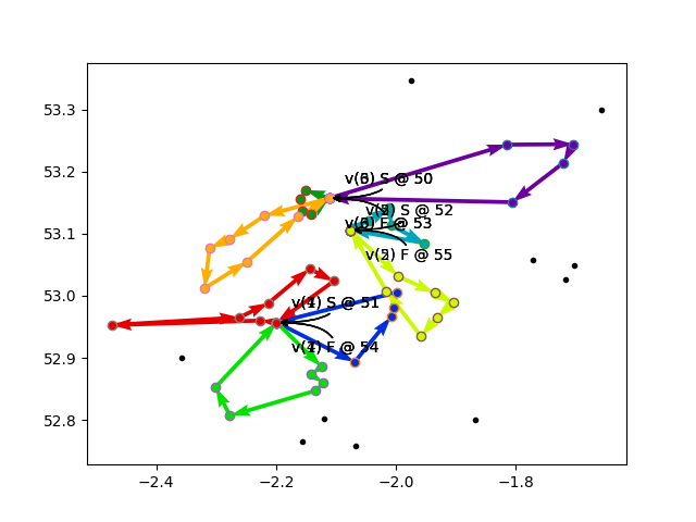
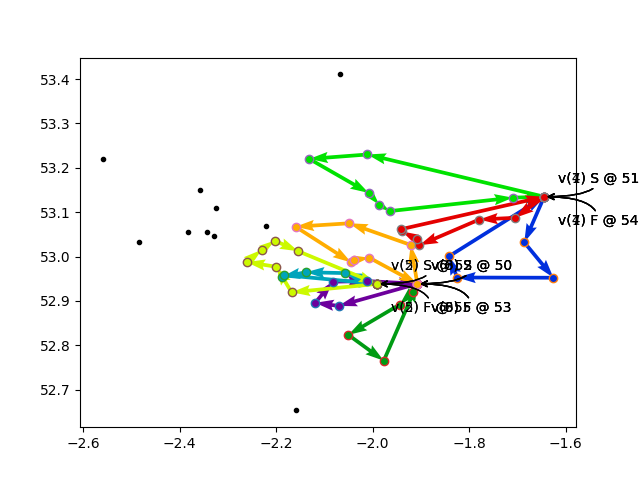
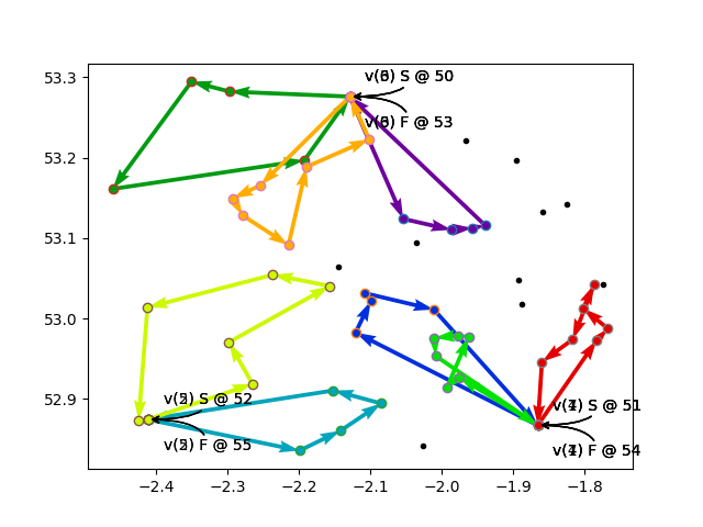
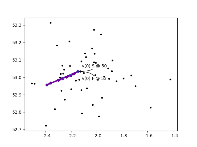
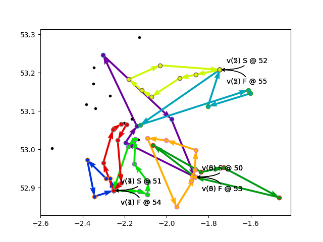
So, to recap. With no disjunctions, all nodes are required, and the model cannot find a solution with 8 vehicles. With a disjunction applied to every customer node, the model can find a solution and drops 10 vehicles. The sample program randomly generates the 50 customer locations and the 3 vehicle depots, and some of the solutions are shown in the three plots below.
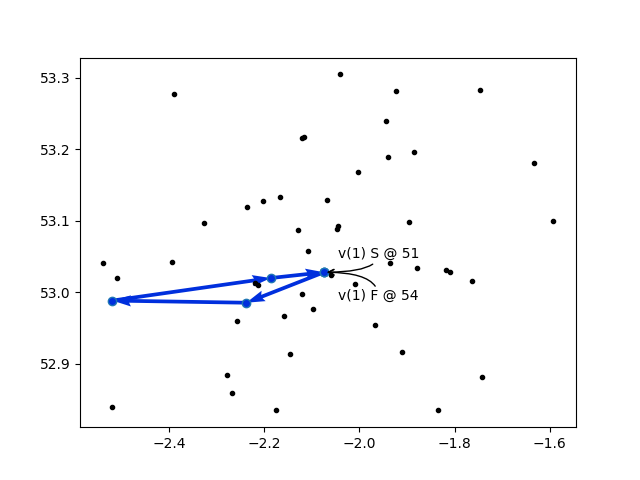
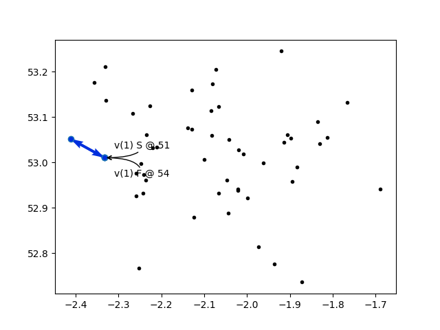
So what happens if just one customer node is given a disjunction?
penalty = 100000  # The cost for dropping a node from the plan.
for cust in customers.customers:
    if cust.index > 0: break
    print('add disjunction to node',cust.index)
    routing.AddDisjunction([int(cust.index)], penalty)
Now, what I expected to happen is that all nodes are required, and just one node is optional. But I was wrong:
...
add disjunction to node 0
succesfully wrote assignment to file /home/user/src/model_assignment.ass
The Objective Value is 139
Route 0: Empty

Route 1: Empty

Route 2: Empty

Route 3: Empty

Route 4: Empty

Route 5: Empty

Route 6: 56 Load(0) Time(0:00:00, 0:00:00) ->  41 Load(0) Time(0:57:56, 5:23:11) ->  0 Load(1) Time(7:15:08, 11:52:23) ->  5 Load(2) Time(8:35:59, 13:13:14) ->  31 Load(3) Time(8:57:00, 13:34:15) ->  22 Load(4) Time(9:06:54, 17:00:39) ->  64 Load(5) Time(10:10:17, 18:59:46) ->  EndRoute 6.

Route 7: Empty


dropped nodes: 1, 2, 3, 4, 6, 7, 8, 9, 10, 11, 12, 13, 14, 15, 16, 17, 18, 19, 20, 21, 23, 24, 25, 26, 27, 28, 29, 30, 32, 33, 34, 35, 36, 37, 38, 39, 40, 42, 43, 44, 45, 46, 47, 48, 49
Vehicle 0 is used False
Vehicle 1 is used False
Vehicle 2 is used False
Vehicle 3 is used False
Vehicle 4 is used False
Vehicle 5 is used False
Vehicle 6 is used True
Vehicle 7 is used False

real	0m0.825s
user	0m0.877s
sys	0m0.434s
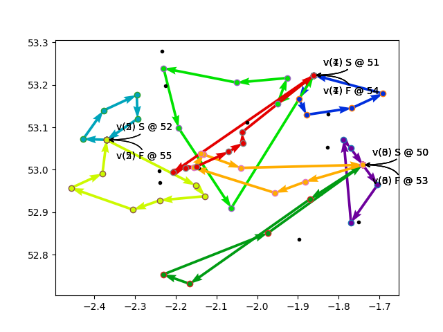
So that is exactly what was observed in practice. With no disjunctions, the solver tries to keep all of the nodes active, and fails. With just one disjunction, it appears that all of the nodes are optional with a drop cost of zero. In some cases as in the above solution, some other nodes are also added in if doing so will not increase the overall cost of the solution. Since the model cost only includes the travel time, not the load/unload time, and because there is rounding error, if stops are reasonably close to the straight line from the depot to the “disjuncted” node, and if the time windows work out correctly, then those other nodes will be opportunistically included. Again, three example plots below indicate some of the random problems I ran.

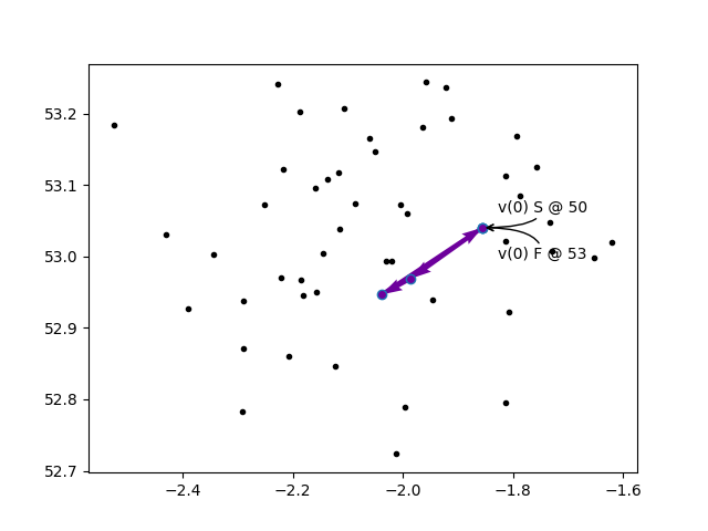
To verify that this is exactly the same as adding a disjunction with zero cost to all nodes but one, I replaced the disjuction loop with the following:
for cust in customers.customers:
    if cust.index < 1:
        print('add optional (pos. penalty) disjunction to node',cust.index)
        routing.AddDisjunction([int(cust.index)], penalty)
    else:
        print('add zero cost disjunction to node',cust.index)
        routing.AddDisjunction([int(cust.index)], 0)
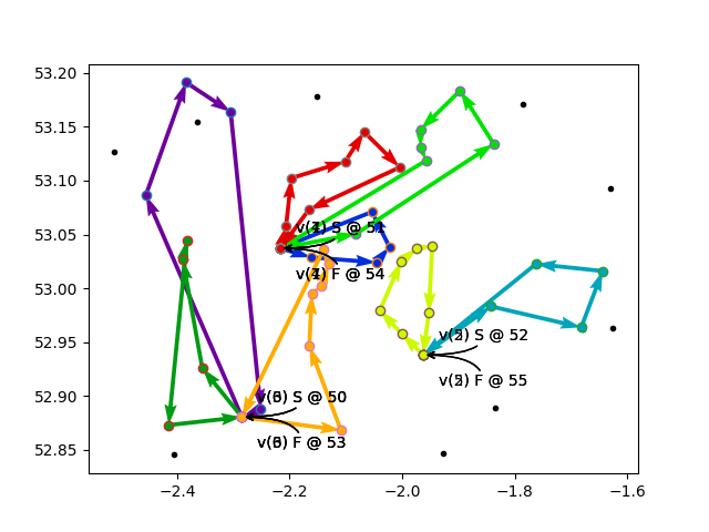
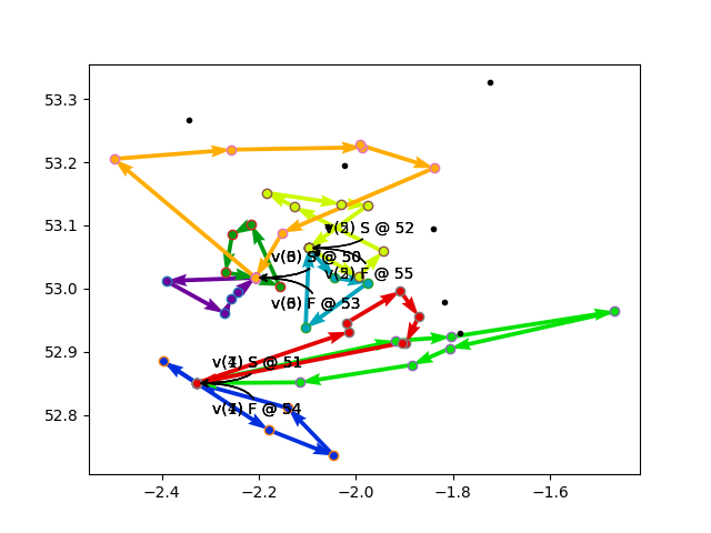
The runs did the same thing as the runs with just one disjuction, as demonstrated by the three example plots below:
Some nodes optional, others required
So how can a disjunction be applied to some stops to make them optional, while still requiring all of the other stops in the final solution? I did a little searching through the issues and found an old, closed issue that linked to the relevant line in the documentation see this comment in the code which is echoed to this page on the documentation site. The one weird trick is to apply a disjuction with a negative penalty. The negative penalty is a flag to the code that tells it to require that particular node be included in the solution.
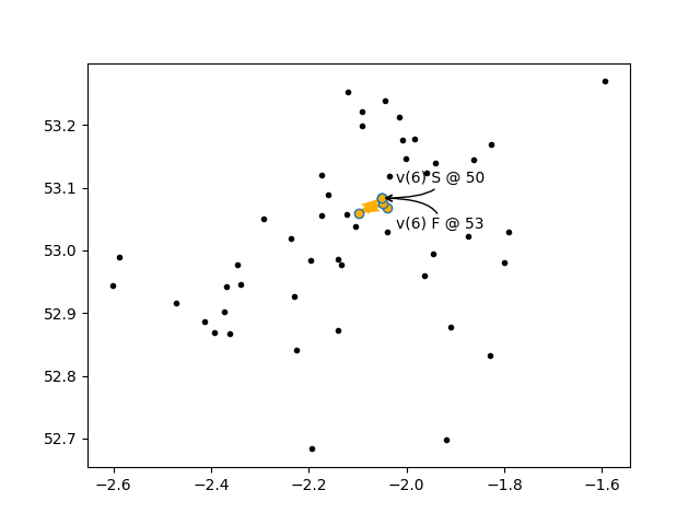
With that in mind, I modified disjunction loop, to make ten
thirty nodes optional, and the rest required using negative penalties.
penalty = 100000  # The cost for dropping a node from the plan.
for cust in customers.customers:
    if cust.index < 30; # 25; # 20; # 15; # 10:
        print('add optional (pos. penalty) disjunction to node',cust.index)
        routing.AddDisjunction([int(cust.index)], penalty)
    else:
        print('add requirement (neg. penalty) disjunction to node',cust.index)
        routing.AddDisjunction([int(cust.index)], -1)
Running that code with just 10 “optional” nodes failed a bunch of times so I gave up and bumped it to 15, then 20, then 25, then 30. After a few runs with 20 required nodes and 30 optional nodes, the solver found a solution that dropped 10 out of the 30 optional nodes.
succesfully wrote assignment to file /home/user/src/model_assignment.ass
The Objective Value is 1001199
Route 0: 50 Load(0) Time(0:00:00, 0:00:00) ->  35 Load(0) Time(1:44:00, 5:48:31) ->  38 Load(1) Time(2:53:48, 6:58:19) ->  48 Load(2) Time(3:35:16, 7:39:47) ->  45 Load(3) Time(7:54:22, 9:06:48) ->  58 Load(4) Time(10:49:32, 18:55:26) ->  EndRoute 0.

...


dropped nodes: 2, 7, 11, 14, 15, 17, 18, 25, 26, 27
Vehicle 0 is used True
Vehicle 1 is used True
Vehicle 2 is used True
Vehicle 3 is used True
Vehicle 4 is used True
Vehicle 5 is used True
Vehicle 6 is used True
Vehicle 7 is used True

real	0m10.876s
user	0m10.958s
sys	0m0.421s
Note that nodes numbered 30 and higher are required, and that the dropped nodes are less than 30, so that is working properly.
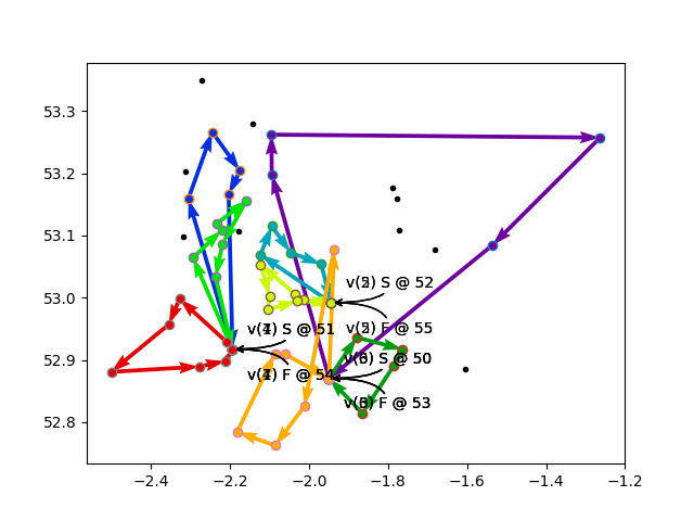
Some other feasible results are below.
Trouble in paradise
I wondered a bit about the reason why I had to bump up the number of “optional” nodes to 30. Invariably, the solver would only drop 10 nodes. I was setting up 50 customers, and the vehicles had a total capacity of 40, so it should be able to drop any 10 nodes.
I convinced myself that the reason the solver was sometimes failing to generate a solution (I ran the program 29 times to generate the 3 valid plots shown above) is that I was randomly requiring 20 out of the 50 nodes, rather than specifically picking 20 nodes that were easy to serve. Those 20 required nodes might have conflicting time windows and locations, thus making the solution infeasible with the 8 vehicles provided.
But, the solver was failing instantly, not making any attempt to search the solution space. It was as if it was running a quick sanity check, and then bailing out when it saw a perceived hard conflict.
I ran into a similar case with my client, but in that case it was clear something was wrong. We had just three customers with optional disjunctions, a few weeks of time to serve them, and one node per day “required” using the -1 disjunction cost. With any one of the three customers excluded, the solver would generate a solution, but with those three customers, it would fail fast.
On a whim, we removed the -1 constraint and instead used a cost of 10. Then the solver would generate solutions with some of the return-home nodes excluded from the solution, for no apparent reason. So we then bumped up the cost of the return-home required nodes to a very high value, 100 times the cost of skipping a customer node, and suddenly the solver had no problem generating a solution.
My guess is that the routing solver has a fast routine that decides if the problem is at all feasible, and if it isn’t, it will fail fast. But in this case, the fail fast result was incorrect; there was a solution, but it required some searching to find it.
So armed with that knowledge, I’ve changed my code to replace the -1 cost with a cost of 10,000,000 for the “required” nodes. The new loop looks like this (note there are just 10 “optional” nodes):
penalty = 100000  # The cost for dropping a node from the plan.
for cust in customers.customers:
    if cust.index < 10:
        print('add optional',penalty,'cost disjunction to node',cust.index)
        routing.AddDisjunction([int(cust.index)], penalty)
    else:
        print('add expensive',penalty*100,'cost disjunction to node',cust.index)
        routing.AddDisjunction([int(cust.index)], penalty*100)
With this change, the solver now consistently would come up with a solution, although occasionally it would drop one of the expensive “required” nodes and quit at the maximum timeout. After bumping up the timeout of the solver run to 2 minutes from 20 seconds, it began to consistently drop just the 10 optional nodes.
For example, look at the following log output of the solver. The initial solution cost is 10,901,362. This tells me that it is dropping nine of the optional nodes as 100,000 cost each, and one of the required nodes with a drop penalty of 10,000,000.
WARNING: Logging before InitGoogleLogging() is written to STDERR
I1109 12:39:19.783761  2093 search.cc:244] Start search (memory used = 111.43 MB)
I1109 12:39:19.785147  2093 search.cc:244] Root node processed (time = 1 ms, constraints = 784, memory used = 111.51 MB)
I1109 12:39:19.792091  2093 search.cc:244] Solution #0 (10901362, time = 8 ms, branches = 34, failures = 0, depth = 33, memory used = 111.54 MB, limit = 0%)
That solution then is improved by the solver over the next few seconds, and then the solver stalled a bit and pondered:
I1109 12:39:19.795251  2093 search.cc:244] Solution #1 (10901355, objective maximum = 10901362, time = 11 ms, branches = 37, failures = 2, depth = 33, neighbors = 1182, filtered neighbors = 1, accepted neighbors = 1, memory used = 111.54 MB, limit = 0%)
I1109 12:39:19.796156  2093 search.cc:244] Solution #2 (10901348, objective maximum = 10901362, time = 12 ms, branches = 41, failures = 4, depth = 33, neighbors = 1203, filtered neighbors = 2, accepted neighbors = 2, memory used = 111.54 MB, limit = 0%)
...
I1109 12:39:46.574213  2093 search.cc:244] Solution #17 (10901295, objective maximum = 10901362, time = 26790 ms, branches = 1324072, failures = 669711, depth = 33, neighbors = 15265, filtered neighbors = 5183, accepted neighbors = 17, memory used = 111.54 MB, limit = 22%)
I1109 12:39:46.601419  2093 search.cc:244] Solution #18 (10901288, objective maximum = 10901362, time = 26817 ms, branches = 1324985, failures = 670161, depth = 33, neighbors = 15266, filtered neighbors = 5184, accepted neighbors = 18, memory used = 111.54 MB, limit = 22%)
Then suddenly, it figures out a route that includes the very expensive node, and the solution cost drops to 1,001,308— one million for the ten dropped nodes with 100,000 cost, and 1,308 for the travel cost between them.
I1109 12:40:29.643079  2093 search.cc:244] Solution #19 (1001308, objective maximum = 10901362, time = 69859 ms, branches = 3513090, failures = 1764496, depth = 33, neighbors = 15317, filtered neighbors = 5235, accepted neighbors = 19, memory used = 111.54 MB, limit = 58%)
I1109 12:40:29.645793  2093 search.cc:244] Solution #20 (1001307, objective maximum = 10901362, time = 69861 ms, branches = 3513127, failures = 1764508, depth = 33, neighbors = 15318, filtered neighbors = 5236, accepted neighbors = 20, memory used = 111.54 MB, limit = 58%)
I1109 12:41:17.691959  2093 search.cc:244] Solution #21 (1001303, objective maximum = 10901362, time = 117908 ms, branches = 5993262, failures = 3004895, depth = 33, neighbors = 17757, filtered neighbors = 5293, accepted neighbors = 21, memory used = 111.54 MB, limit = 98%)
I1109 12:41:19.783864  2093 search.cc:244] Finished search tree (time = 120000 ms, branches = 6004660, failures = 3013849, neighbors = 24871, filtered neighbors = 7518, accepted neigbors = 21, memory used = 111.54 MB)
I1109 12:41:19.784078  2093 search.cc:244] End search (time = 120000 ms, branches = 6004660, failures = 3013849, memory used = 111.54 MB, speed = 50038 branches/s)
succesfully wrote assignment to file /home/user/src/model_assignment.ass
The Objective Value is 1001303
...


dropped nodes: 0, 1, 2, 3, 4, 5, 6, 7, 8, 9
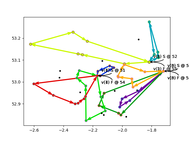
This solution is shown in the left hand plot, below.
Another run was even more exciting. The solution starts off dropping two of the very expensive required nodes:
I1109 13:05:25.485968  2097 search.cc:244] Start search (memory used = 111.43 MB)
I1109 13:05:25.487123  2097 search.cc:244] Root node processed (time = 1 ms, constraints = 784, memory used = 111.51 MB)
I1109 13:05:25.493994  2097 search.cc:244] Solution #0 (20801324, time = 7 ms, branches = 34, failures = 0, depth = 33, memory used = 111.54 MB, limit = 0%)
...
I1109 13:05:30.043107  2097 search.cc:244] Solution #21 (20801240, objective maximum = 20801324, time = 4557 ms, branches = 20991, failures = 16598, depth = 33, neighbors = 16743, filtered neighbors = 4511, accepted neighbors = 21, memory used = 111.54 MB, limit = 3%)
Then the solver output stalled while the solver considered its options. With a burst of activity at 41 seconds in, it managed to drop one of the expensive nodes! The solution was now clocking at 10,901,311:
I1109 13:06:07.091540  2097 search.cc:244] Solution #22 (10901311, objective maximum = 20801324, time = 41605 ms, branches = 2144681, failures = 1082838, depth = 33, neighbors = 19920, filtered neighbors = 7624, accepted neighbors = 22, memory used = 111.54 MB, limit = 34%)
...
I1109 13:06:56.192648  2097 search.cc:244] Solution #36 (10901277, objective maximum = 20801324, time = 90706 ms, branches = 4783483, failures = 2402502, depth = 33, neighbors = 27211, filtered neighbors = 7695, accepted neighbors = 36, memory used = 111.54 MB, limit = 75%)
So I thought this was going to be my counter example—a case that the solver failed to drop just the 10 optional nodes. But then at 97 seconds (out of a max of 120) the solver made it over the hump:
I1109 13:07:03.215325  2097 search.cc:244] Solution #37 (1001334, objective maximum = 20801324, time = 97729 ms, branches = 5015790, failures = 2522901, depth = 33, neighbors = 30753, filtered neighbors = 10773, accepted neighbors = 37, memory used = 111.54 MB, limit = 81%)
I1109 13:07:03.218006  2097 search.cc:244] Solution #38 (1001321, objective maximum = 20801324, time = 97731 ms, branches = 5015810, failures = 2522904, depth = 33, neighbors = 30754, filtered neighbors = 10774, accepted neighbors = 38, memory used = 111.54 MB, limit = 81%)
I1109 13:07:25.486315  2097 search.cc:244] Finished search tree (time = 120000 ms, branches = 6122780, failures = 3076579, neighbors = 30780, filtered neighbors = 10800, accepted neigbors = 38, memory used = 111.54 MB)
I1109 13:07:25.486541  2097 search.cc:244] End search (time = 120000 ms, branches = 6122780, failures = 3076579, memory used = 111.54 MB, speed = 51023 branches/s)
succesfully wrote assignment to file /home/user/src/model_assignment.ass
The Objective Value is 1001321
Route 0: 50 Load(0) Time(0:00:00, 0:00:00) ->  22 Load(0) Time(11:21:16, 11:56:40) ->  11 Load(1) Time(12:31:02, 13:06:26) ->  41 Load(2) Time(14:46:03, 15:21:27) ->  38 Load(3) Time(15:17:13, 16:44:07) ->  58 Load(4) Time(15:50:54, 18:49:46) ->  EndRoute 0.

...

dropped nodes: 0, 1, 2, 3, 4, 5, 6, 7, 8, 9
This solution is the center plot, below.
Eventually I finally did hit a case where dropping one of the
“required” nodes was unavoidable. The final cost was 10,901,320 after
just 55 seconds of search time out of the allowed 2 minutes. The
solver dropped nodes dropped nodes: 0, 1, 2, 4, 5, 6, 7, 8, 9, 33.
This solution is shown in the right hand plot, below. The far-flung
nodes and poor placement of depots probably contributed to the failing
case.
So the moral of the story is, if you have just one or two nodes that aren’t going to conflict with whatever quick look the solver does to assess the overall feasibility of the problem, then great! It is probably safe to use a disjunction cost of -1 to force those nodes to be required. However, if the solver fails instantly without even trying, then chances are using a disjunction cost of -1 to require a node is a bad idea. Instead, try bumping up the cost of the required nodes to something really high, along with potentially increasing the timeout of the solver.